Gaussian Quadrature - Gauss Legendre Integration
Often in the field of quantitative finance, it is required to apply numerical integration to arrive at the risk or valuation numbers which would otherwise not be possible as closed form solutions to these integrations dont exist. There are a few choices of numerical methods available to achieve this. Examples include Trapezoidal, Boole's and Gaussian quadratures. Gaussian quadrature is probably the most popular method in practice today. This article focuses on Gauss Legendre integration which is applied to calculate definite integrals numerically.
Let us first first briefly talk about Legendre polynomials:
Legendre polynomials
Consider the recursive equations 1 and 2 below.
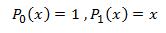
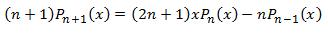
Applying equation 2 for n = 1, we get 2P2(x) = 3xP1(x) - P0(x) (3)
Solving (3) we have , 
Similarily, for n = 2, we get 3P3(x)=5xP2(x)-2P1(x) or, 3P3(x)=15/2x2-5/2x-2x
which leads to, 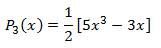
The first five legendre poynomials are tabulated below
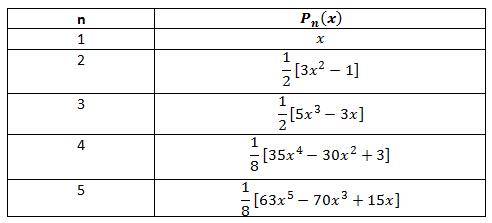
Table 1: The first five legendre polynomials
Roots of Legendre functions
There are quite a few solver algorithms that can be used to find the root of a polynomial. These include methods like Bisection, Newton, Brent etc. Here we, however, need a scheme to calculate all roots to these Legendre polynomials. Following is a suggestive scheme:
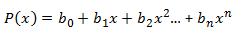
Assume we have a legendre polynomial P(x), we need all roots such than P(x) = 0.
1. Find the first root (R1) of P(x) using a solver (Bisection, Newton etc.)
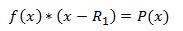
2. Find the polynomial f(x) such that f(x) * (x-R1) = P(x).
3. Use the solver to find the next root (R2).
4. Find f'(x) such that f'(x) * (x-R2) = f(x) or, (x-R1) * (x-R2) * f'(x) = P(x)
So on an so forth..
Tip: While using Newton's method some authors suggest using x = Cos(Pi * (4 * i + 3) / (4 * n + 2)) where i is the root number, and n is the polynomial degree. This initial guess converges efficiently.
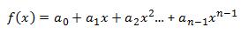
Evaluating f(x) such that f(x) * (x - R1) = P(x)
Say we have
 (1),
(1),
 (2)
(2)
 (3)
(3)
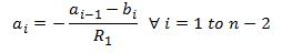
and we need to find out the coefficients a0, a1, a2, a3...etc.
solving (3) we get,

which simplifies to
 , (4)
, (4)
 and, (5)
 (6)
(6)
2 point Gauss Legendre Integration rule
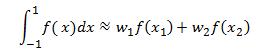
The two point Gauss Legendre Integration rule is shown in the equation (7) below:
 (7)
(7)
where x1 and x2 are the abscissas and w1 and w2 are the weights for the 2 point Gauss Legendre Integration rule. The abscissas for a n point rule are the roots of the Legendre function of degree n. As an example, for a 2 point rule we have the Legendre function 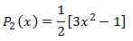 . The roots of the equation P2(x) = 0 are hence the abscissas for the 2 point Gauss Legendre rule.
Going further, the roots of the Legendre function of degree 2 (see table 1 above) are as shown below.
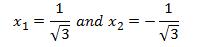 (8)
(8)
To find the weights w1 and w2 , we need two relationship equations. So we use our knowledge of definite integration of 1 and x which gives us the following two relationships.
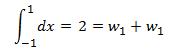 (9)
(9)
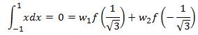
or, 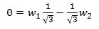 (10)
(10)
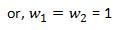 (11)
(11)
Substituting (11) in (7) we get
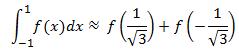 (12)
(12)
Application of 2 point Gauss Legendre rule
Example 1:
Let's take 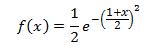 so that the two point Gauss Legendre approximation is as follows:
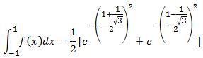
or, 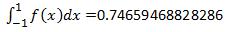
where the exact solution is 0.74682413281243
Example 2: Evaluate 
The two point rule leads to 
so that the approximate solution using two point rule is 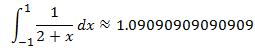
where the exact solution is ln(3) - ln(1) = 1.09861228866811.
4 point Gauss Legendre Integration rule
Abscissas and weights for the 4 point rule are as follows:
x1 = -0.339981043584856, x2=-0.861136311594053, x3=0.339981043584856 and x4=0.861136311594053.
w1 = 0.652145154862546, w2 = 0.347854845137454, w3 = 0.652145154862546 and w4 = 0.347854845137454.
Example 3: Let us revisit the second example so that we need to evaluate  using the 4 point Gauss Legendre rule.
Applying the four point rule we have 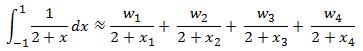
Substituting the values of weights and abscissas specified above we get 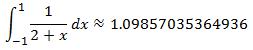 . We notice that the 4 point rule yields a closer result than the 2 point rule.
N point Gauss Legendre Integration rule
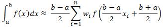
So far we have seen the application of 2 and 4 point Gauss Legendre integration rules. A generalisation for a higher order integration rule is as follows: 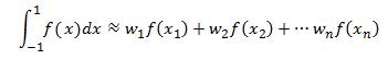 (13)
(13)
where xis and wis are the abscissas and the weights applicable for the N point rule. A table for higher order Gauss Legendre rule is available in the link below.
View Gauss Legendre abscissas and weights of higher order Gauss Legendre quadratures.
A higher order rule generally gives a better approximation to the required integration. Table 2 below shows how the results improve for the calculation of  as we move to higher order Gauss Legendre rules. A 32 or 64 point rule is sufficient for most real life cases.
| Order (n) | Gauss Legendre approximation | Error (%) |
|---|---|---|
| 2 | 1.09090909090909 | 0.70118% |
| 4 | 1.09857035364936 | 0.00382% |
| 8 | 1.09861228751918 | 0.000000105% |
| 16 | 1.09861228866810 | 0.0000000000011% |
Table 2: A comparison between different orders Gauss Legendre quadrature.
Change of intervals for definite integrals
Any definite integral over [a,b] can be changed to an integral over interval [-1,1] using the following formula:
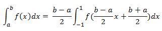
Hence to calculate the definite integral over any arbitrary bounded range [a,b] use the following formula:
where xis and wis are the abscissas and the weights applicable for the N point rule.
Singularities and Gauss Legendre Integration
If there are singularities in the bounds [a,b], the fixed point Gauss Legendre rule may lead to incorrect results and hence must be avoided. As an example  , the exact solution is -2 whereas the two point rule leads to the answer 6.