Markov and Martingale processes
This article introduces the concepts of martingale and markov processes and their application in derivatives option pricing. The text assumes a simple discrete time binomial model framework.
Martingale process
Any martingale process is a sequence of random variables that satisfies
 .....(1)
The discounted stock price under the risk neutral probability measures is a martingale process. The risk neutral probabilities are chosen to enforce the fact. i.e.
 .....(2)
here the  indicates the expected value under risk neutral measure.
Lets take a one period process, the stock price  can either go to either
  with a risk neutral probability
  or
or  with a probability
  [u>1+r>d]. It is important at this stage to distinguish the risk neutral probabilities from the actual probabilities. This framework is based on the risk neutral premises [i.e it uses risk neutral probabilities] which determines the fair value of the option based on its hedging costs.
 ......(3)
so that p solves to ,
 ...(4) and
 ....(5)
with continuous discounting these formulas become
 ...(4a) and
 ....(5b)
Its straightforward to see that we get the same results for an n period process as well. What the result means is that the discounted stock price [or forward price] for the (n+1)th period depends only on the stock price of nth period.
Markov property
Within the binomial asset pricing model. Let X0, X1,....XN be a random process. If for every n between 0 and N-1 and f(x), there exists another function g(x) such that
 ....(6)
We say that X0,X1...XN is a Markov process.
Again what this means is that the information required to evaluate  is available in XN i.e the path that the variable took to get to XN is not required. What this means in terms of derivatives option pricing is that we do not need to save the path information when the option payoff is Markov. On occasions we encounter non Markov processes. As an example consider an Maximum to date payoff for the option. The option payoff for the nth period not only depends on the stock price at the nth period but also the path taken to get to it. When we encounter these non-Markov processes we sometimes recover the Markov property by adding one or more so called state variables. [for example in this case the extra variable stores during maximum till date stock price]
Martingale is a special case of Markov wth f = x and g = x. However for the process to be Markov we require for every function f a corresponding function g such that (6) holds. So not all Martingales are Markov. Similarly not all Markovs are martingales. The function g required to make the process Markov need not necassorily be x.
Risk Neutral Pricing
We continue the discussion of risk neutral premises. One might wonder why risk neutral probabilities as opposed to actual probabilties lead to fair option values. To answer this lets assume a european call option under a two period binomial model framework. The arguments that we present would be applicable to a multi period framework as well.

Lets assume that the initial stock price is 1 and u = 2 and d = 1/2 so that after first period the stock price can take either 2 or 1/2 so on an so forth. See the image below. Also lets assume that the interest rate is 10%. i.e. r=0.1. The strike of the european call option is 1.
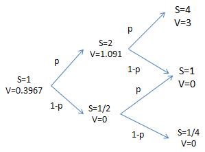
Using equations (4) and (5) we get the risk neutral probabilities p = 0.4 and 1-p = 0.6. Under the risk neutral pricing framework, it is possible to construct a riskless portfolio that yields the same option payoff which therefore can be used to hedge the option. From the figure above, we take the fair price of the option as the expected payoff under the risk neutral measure equating to 0.3967. This is the amount that the seller of the option receives as premium at period 0 as the cash component. The seller delta hedges at the end of each period by either buying or selling underlying stock using the available cash or borrowing if need be. The discrete risk free rate is 10% which will also be the borrowing cost.
The amount of stocks at the end of each period [=delta] is calculated using the formula 
So that at period 0 the seller would buy n = (1.09091 - 0)/(2 - 0.5) = 0.7273 stocks with (0.7273 - 0.3967) = 0.3306 borrowed cash. [option premium cash already available to him]
At the end of first period the stock either goes to S = 2 or 0.5. The seller now owes cash = (1+r) 0.3306 = 0.3636 cash due the interest accrued on the borrowed cash. Let us now assume that the stock ended at S = 2 after the first period. He will again readjust the amount of stocks to n = (3 - 0)/(4 - 1) = 1. He already owns 0.7273 stocks. He purchases rest of (1 - 0.7273) = 0.2727 shares using 2 * 0.2727 = 0.5455 more cash. So that he now owes 0.5455 + 0.3636 = 0.9091 in all and owns n= 1 stock at the end of period 1.
Given that the stock was S = 2 at the end of period 1, we now show that irrespective of whether the stock rises to S = 4 or goes back 1 he will have enough resources to settle the call option contract. Given the interest accrued on the borrowed money in period 2, the seller now owes cash = 0.9091 * (1+r) = 1. He owns n =1 share from period 1. If now the stock rises to 4, he needs to pay the buyer payoff = 4 - 1 = 3 so that he pays 3 to the buyer and using the remaining 1 he pays off the borrowed money.
We can do a similar analysis for the stock price S = 0.5 at the end of the first period but is left to the reader. We found that the option price calculate using risk neutral probabilities yields enough resources to be able to complete hedge the option. We hence conclude this article by emphasing that in the risk neutral premises its possible to construct a riskless portfolio that yields the same payoff as the option and hence the fair price of the option should be the price calculated using the risk neutral probabilities [law of one price otherwise we can contruct an arbitrage portfolio].


